Concepts of Depth-wise separable convolution

I read "MobileNets: Efficient Convolutional Neural Networks for Mobile Vision Applications" by Andrew G. Howard, Menglong Zhu, Bo Chen, Dmitry Kalenichenko, Weijun Wang, Tobias Weyand, Marco Andreetto, Hartwig Adam
to understand Depth-wise separable convolution, and i'm going to organize key concepts about that.

1. Purpose
2. Standard Convolution
3. Depth-wise Separable Convolution
4. Result

1. Purpose

The purpose of the paper is making light weight Deep Neural Network(in terms of computation).
To achieve that goal, they introduce Depth-wise separabel Convolution and Single global hyper-parameters which efficiently trade off between latency and accuracy.
This article deals with Depth-wise separable convolution.

2. Standard Convolution

like above image, standard convoluion filters are applied to all channel of input , and each filter makes separate output channel, where $M$ is a number of input channels, $N$ is a number of output channels and $D_k \times D_k$ is kernel size of a filter.

Thus, the standard convolutions have the computational cost of:
$D_k \times D_k \times M \times N \times D_F \times D_F$
where $D_F \times D_F$ is a size of input feature map.

3. Depth-wise Separable Convolution

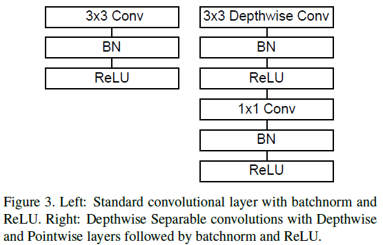
Depth-wise separable Convolution consists of two types of layers.
each layer is followed by BatchNorm and ReLU like right one of above image.

• Depth-wise conv
  • do convolution using one filter per input channel so that number of output channel is same as input
  • this separates each channel of input not mixing it.
• Point-wise conv
  • do linear combination of the output of depth-wise conv with 1x1 conv
  • by doing this, you can control output dimention

3.1. Depth-wise conv

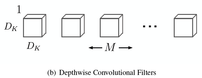Like above image, Depthwise convolutional filters applied each input channel not mixing them.
In the image, $D_k \times D_k$ is kernel size of a filter and $M$ is number of channel(input and output are same).

Thus, computational cost is:
$D_k \times D_k \times M \times D_F \times D_F$
where $D_F \times D_F$ is a size of input feature map.

3.2. Point-wise conv

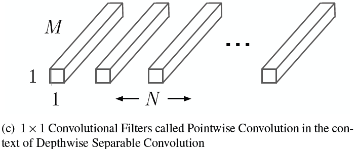
In the image, $M$ is a number of input channel and $N$ is a number of output channel.
as you can see, this is for linear combination of input channels to fit to number of output channels.

Thus, computational cost is:
$M \times N \times D_F \times D_F$
where $D_F \times D_F$ is a size of input feature map.

4. Result

computational cost
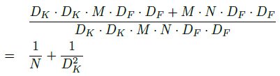above expression is a result of dividing cost of Depth-wise separable conv by cost of Standard conv.
as you can see, Depth-wise separable conv is computationally efficient.

accuracy
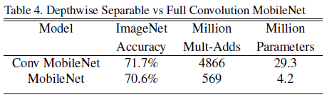above table shows comparison of accuracy between standard conv(Conv MobileNet) and Depth-wise separable conv(MobileNet).
There seems to be Pros and Cons between computational efficiency and accuracy.